Plot a phylomorphospace for a component from an analysis of multiple data blocks

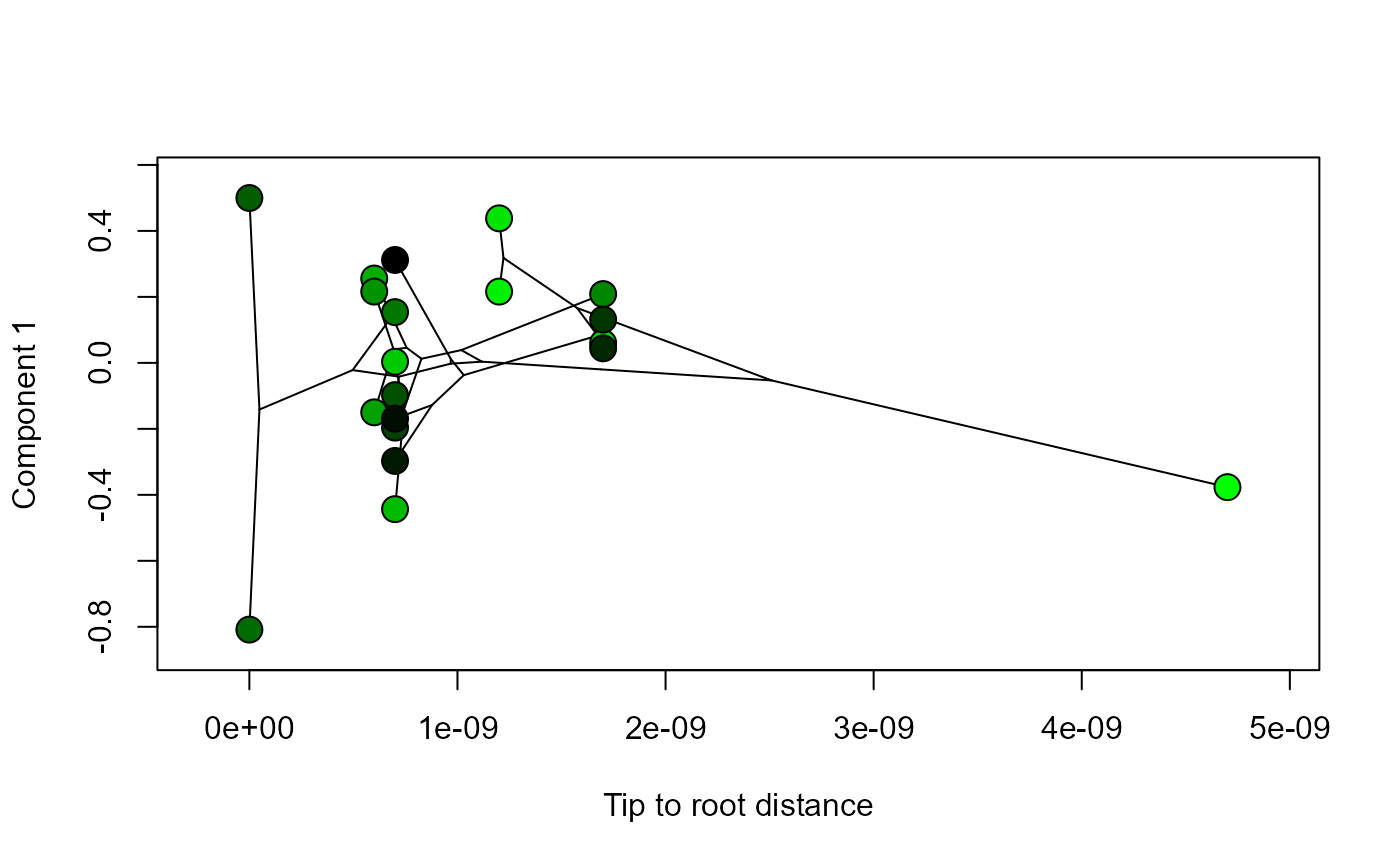
A plot to visualise the evolutionary relationships between specimens that are represented by values projected into a morphospace (e.g. Sidlauskas, 2008). Here the projected values are from a single component from an analysis of multiple data blocks. Rather than generating a two- or three-dimensional morphospace, this function plots consensus or principal component values against tree distance to show changes in the component value across the evolutionary history of the clade. The component values that are visualised using this function will either be from 1) the consensus space of an analysis performed with Regularized Consensus Principal Component Analysis, or 2) will be from an analysis of a superblock (i.e. column-wise concatenation of individual data blocks) if principal component analysis was performed instead.

phylomsPlot(
  result,
  phy,
  n.names,
  comp = 1,
  pcol = NULL,
  xlab = "Time (Ma)",
  label = "off",
  fsize = 0.8
)

Arguments

result	result produced by the `analyseBlocks` function.
phy	a phylogenetic tree (class “phylo”) with `n` tips, where `n` is the number of samples in each block. Tip labels must be included and must correspond to the names of the samples in each block.
n.names	a vector of character strings where entries in the vector represent names of the `n` samples present in each block. IMPORTANT NOTE: The sequence of character strings in `n.names` must match the sequence that samples are named in each block, and the names must exactly match the tip labels in the phylogenetic tree. For example, consider a block containing data from five samples where the first, second and third rows of the block contain data from samples "A", "B" and "C", and the fourth and fifth rows contain data from samples "D" and "E". Consequently, 1) `n.names = c("A", "B", "C", "D", "E")`, 2) `phy` should only include five tips, and 3) `phy$tip.labels` should be "A", "B", "C", "D" and "E" (in any order).
comp	the component selected to be shown in the phylomorphospace plot. Default is component one. The selected component must be within the range of components calculated by `analyseBlocks`.
pcol	optional colour value (integer, hex code, colour name) or vector of colour values to be applied to the points in the phylomorphospace plot. If no value is specified then points will be coloured in a gradient from black to green according to their sequence in the data blocks. If a single integer is supplied (e.g. `pcol = 1` or `pcol = "red"` or `pcol = "#ffffff"` then all points will have the same colour. If a vector of length n is supplied (e.g. `pcol = 1:10`) then each point will be coloured by a value corresponding to its position in the vector.
xlab	character string displayed along the horizontal axis of the phlyomorphospace plot. Default is "Time (Ma)".
label	a logical value indicating if the points in the phylomorphospace should be labelled using `n.names`. Default value is `off` (i.e. names are not shown).
fsize	size of the `n.names` labels if they are included in the plot. Default is 0.8.

Details

phylomsPlot helps to visualise the result from the analyseBlocks function by presenting an evolutionary context for score values from a consensus space (for option = "rcpca" in analyseBlocks) or from a concatenated superblock (for option = "pca" in analyseBlocks). phylomsPlot is a wrapper for phylomorphospace from the phytools package (Revell, 2012), which is in turn based on the projection of a phylogenetic tree into a morphospace by Sidlauskas (2008). The function phylomsPlot uses the distRoot function from the adephylo package (Jombart et al. 2010). phylomsPlot does not specifically use functions from the ape package (Paradis et al. 2004), but this package may be called to read phy into R.

References

Jombart T, Balloux F, Dray S. 2010. adephylo: new tools for investigating the phylogenetic signal in biological traits. Bioinformatics 26: 1907–1909 https://doi.org/10.1093/bioinformatics/btq292

Paradis E, Claude J, Strimmer K. 2004. APE: Analyses of phylogenetics and evolution in R language. Bioinformatics 20: 289–290 https://doi.org/10.1093/bioinformatics/btg412

Revell LJ. 2012. phytools: An R package for phylogenetic comparative biology (and other things). Methods in Ecology and Evolution 3: 217–223 https://doi.org/10.1111/j.2041-210X.2011.00169.x

Sidlauskas B. 2008. Continuous and arrested morphological diversification in sister clades of characiform fishes: a phylomorphospace approach. Evolution 62: 3135–3156 https://doi.org/10.1111/j.1558-5646.2008.00519.x

Examples

# Simulate a phylogenetic tree with 20 tips
library(phytools)
#> Loading required package: ape
#> Loading required package: maps
phy <- pbtree(b = 0.1, n = 20)

# Simulate, combine and analyse two data blocks with 20 samples each
block1 <- dodecBlock(n = 20)
block2 <- dodecBlock(n = 20)
blocklist <- combineBlocks(blocks = c(block1, block2))
result <- analyseBlocks(blocklist)

# Simulate a vector of names (here just use the tip labels)
n.names <- phy$tip.label

# Generate phylomorphospace plot
phylomsPlot(result, phy, n.names, comp = 1, xlab = "Tip to root distance")